NOCTIS ARRAY archive
Pipeline · viewer · object guides
FROM RAW EXPOSURES TO A LINKED TRACK.
Nine pages, one pipeline, read in order. The table below walks the sequence in the order it actually runs — why the same patch of sky gets photographed over and over, how those exposures get pinned to one shared pixel grid, how subtracting a reference reveals what changed, and how each change gets measured, classified and, for the fast-moving ones, linked into a track. The last three entries show how to read the site's own viewer and give full guides to the two object types the pipeline actually finds. Each row opens as its own page. Read them in order — each one assumes the one before it.
Unlike the Overview page, nothing in this section is invented. Every tutorial below describes the real pipeline — the same one the viewer, survey and cell browsers actually run.
Nine tutorials, read in order.
Each one opens as its own page. The first seven walk the pipeline itself, start to finish; the last two are full guides to the two object types the pipeline actually classifies.
Acquisition
Why a single exposure is never enough, and why ZTF revisits the same patch of sky over and over.
Subtraction
Matching blur and brightness first, then subtracting a reference to reveal only what changed.
Detection
Every blob above the noise gets a position, a brightness, a shape, and a 63×63 px stamp.
Classification
A pretrained CNN grades every detection real or bogus, then a second pass guesses what it is.
Motion
A fast mover draws a line instead of a point — the separate branch that cascades and links it into a track.
Reading the viewer
Every layer, marker, and drawer in the site's own difference-image viewer, mapped back to a step above.
One field, not a ceiling. Field 468 — the worked example running through tutorials 01–07 — is not a limit of the method. The same code has since been generalized into a survey harvester that sweeps many fields and many nights; browse what it's found so far on the Survey page.
Reading a difference image, and the cutout behind every detection.
Tutorial 03 explains how the subtraction is done and tutorial 04 how the leftovers are measured. This is the practical half: what the pictures in the browsers actually mean when you open one.
Amber appeared. Cyan faded. Black stayed the same.
A difference image is not a photograph of the sky — it is a photograph of the change. A deep reference image of the same patch has already been subtracted, so every star that held still cancels to nothing, and empty sky is drawn true black on purpose. The same amber-up / cyan-down language is used everywhere on this site: the viewer's change overlay, the per-cell stacks, the survey markers, and the cutouts below.
Flux appeared or brightened here since the reference was built.
Flux faded — the source was brighter in the reference than it is now.
Nothing changed, or the change sits below the display's noise floor. The measurements themselves are made on the full, unfloored data.
Four shapes are worth recognising. A compact blob is the interesting one — something genuinely changed brightness at a fixed position. A line is something that moved during the exposure, and feeds the motion branch of tutorial 06. Amber and cyan side by side, as a pair or a ring, is a dipole: two images that were not aligned to a perfect sub-pixel match, so the subtraction left one edge over and the other under — an artifact, not a fading star, and a documented limit of this pipeline. A hollow black core with wings is a saturated star, whose centre carried no usable information in either image.
Every detection now carries its own cutout.
Click any detection anywhere in the application — a marker on a map, a row in a list — and a drawer opens with a cutout: a small square of real sky, cut from the very images the measurement was made on, centred on that detection's own position. Each panel is 63 × 63 pixels, the same stamp size ZTF publishes in its own alerts, and every panel is stretched by the same measured noise level of the whole frame — not by its own brightest pixel — so two cutouts can be compared honestly against each other.
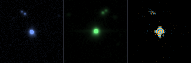
This night. The single exposure the detection was made in — the "after".
Before. ZTF's deep co-add of the same sky from many earlier visits, so it is far quieter than any one night.
What changed. Reference subtracted from science, in the colour key above.
The caption under a cutout always names the panels it actually has, and it will not always say three: most of the harvest ran in a motion-only mode that never downloads a science frame, so many detections carry a reference-and-difference pair, and some the difference alone. That is a fact about which images exist for that exposure, not a judgement on the detection — read the caption rather than assuming a triplet. Read the panels left to right, then the verdict beside them; the picture and the classification are two independent opinions, and a cutout that looks nothing like a star is a good reason to distrust a confident-sounding label.
Three places to see difference images. The difference viewer shows one worked field in depth; every sky cell has its own viewer with one difference image per visit, steppable and blinkable; and the survey map loads each cell's real imagery once you zoom in far enough. The viewer guide walks every control on all three, with more worked cutout examples.
Go watch it run.
Everything above is the real pipeline, explained in the order it runs. The browsers below are that same pipeline's actual output — a working ZTF difference-imaging system, not a mockup of one.
Or read what this project actually is