Our pipeline · difference viewer
then keep it open in a tab
VIEWER
GUIDE.
The difference viewer packs a lot into one screen: an image stack, a tuning panel, three floating side-panels and a detail drawer. Nothing on it is decoration — every panel maps to a real, documented part of the pipeline. This page walks through what each piece is, where it lives on screen, and what it's showing you — including how to read a difference image itself, and the per-detection cutouts now attached to every row in the application — so the first few minutes in the viewer are orientation instead of guesswork.
The five things you need before anything else
If you open the viewer right now and do nothing else, this is everything you need to look around and find something interesting.
- Drag to pan, scroll (or the −/+ buttons) to zoom. The view boots wide on the real sky, then flies in on the one ZTF field this page is built from — give it a few seconds to land.
- Click any coloured marker (a reticle or bracket on the image) to open a detail drawer on the right with that detection's thumbnail and verdict.
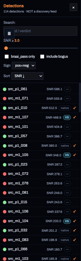
- Press L or click the ≡ button (top-left) to open the full, filterable list of every detection in this field.
- The display button (top-right toolbar) is where you turn image layers on/off and adjust brightness/contrast — see Toolbar & display panel below.
- If the page just shows an error about a local server, you opened the
file directly. Run
./serve.shfrom the project root and reload — see Troubleshooting.
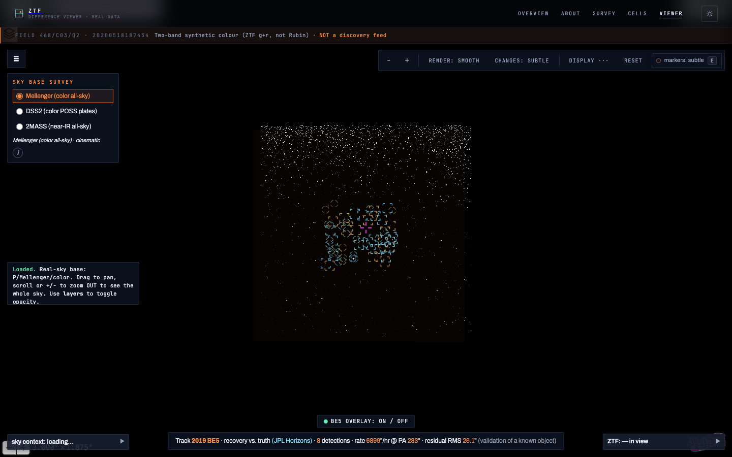
This is one ZTF exposure, run through our own pipeline. Not a discovery feed.
Every marker on the map is a detection our own difference-imaging and classification code produced — not an official ZTF alert, not a confirmed astronomical event. Three honest outcomes exist and the viewer is careful to keep them distinct: a recovery is a known, catalogued object our pipeline found blind (a validation of the detector, not news); a candidate is unconfirmed and, on a single field like this one, usually an artifact; a verdict is a real/bogus + object-type classification from the stationary branch. Where a branch never ran, it reads not run — never "bogus."
The colour in the sky image is synthetic: ZTF has two public optical bands (g and r), so red = r-band flux, blue = g-band flux, and green is a blended mix of the two — not a third real filter. This is ZTF data, not Rubin/LSST. And the whole page is baked around one field and one exposure (named in the strip at the very top of the viewer) — for the wider harvest across many fields and nights, see Survey and Cells.
Where everything lives
A schematic of the viewer's own screen, at the same corners the real controls sit in. Every labelled zone below has its own section further down this page.
What's actually stacked on screen
The map is several images layered on top of each other. You rarely need to think about this — but when something looks unexpected, this is the first thing to check in the display panel's Layers list.
the photographic backdrop
Many aligned exposures of this field median-stacked together (deep, low-noise), one stack per band. Red = r-band, blue = g-band, green = a synthetic blend of both. If the deep stacks weren't built, a single-epoch science frame is shown instead (in grayscale) — the Layers panel names whichever is active.
the actual detector output
One exposure's science frame minus a deep reference template. Amber/warm = flux appeared or brightened; cyan/cool = flux faded, or an alignment "dipole" artifact. Transparent = below the noise floor, i.e. nothing changed. Subtle (30% opacity) by default so the sky stays the hero — the toolbar's changes button floods it back to full strength.
the "before" reference
The deep, multi-epoch co-add that the change overlay was subtracted against. Hidden by default; the blink button in the display panel toggles between it and the current sky every 0.7 s — the classic astronomer's trick for spotting a change by eye.
context, not our data
An all-sky survey (not ours) shown behind the ZTF imagery when you zoom out past our field's footprint, or when sky ctx is switched on. Off by default so empty sky renders true black instead of a survey haze. Choose which survey via the sky-base picker.
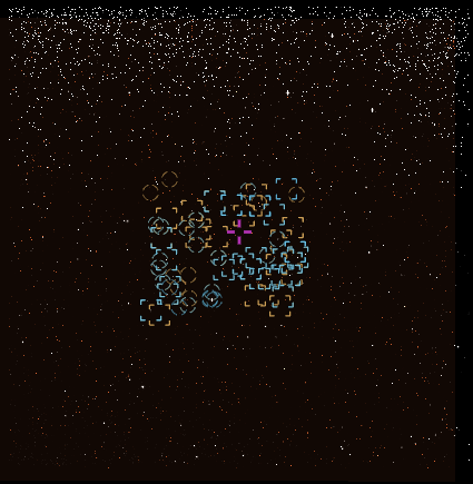
How to read a difference image
A difference image is not a photograph of the sky — it is a photograph of the change. A reference image of the same patch has already been subtracted, so every star that stayed exactly the same cancels to nothing. What is left is what moved, appeared, faded — plus whatever the subtraction failed to cancel cleanly. Learning to tell those two apart is most of the skill.
That amber-up / cyan-down language is the same on every surface of this site — the change overlay here, the per-cell stacks, the survey map's markers, and the cutouts in section 08.
Four shapes worth recognising
One tight amber (or cyan) knot the size of a star image. This is the interesting case: something genuinely changed brightness at a fixed position — a variable star, an AGN, a transient.
An elongated smear. Something moved far enough during the exposure to draw a trail instead of a point — a fast asteroid, or a satellite. This is what feeds the pipeline's separate motion branch.
A dipole — a bright-and-dark pair, or a ring, on a star that did not really change. The two images were not aligned to a perfect sub-pixel match, so subtraction left one edge over and the other under. An artifact, and a well-documented limit of this pipeline — not a fading star.
A saturated star. Its centre pegged the detector's maximum in both images, so the centre carries no usable information and subtracts to a black hole ringed by leftovers. Always an artifact.
One star can produce two rows. Detection runs over the positive difference and the negative difference separately, so a dipole is frequently catalogued twice — once as a sign +1 detection and once as sign −1, at sky positions less than an arcsecond apart. If two entries in a list sit on top of each other with opposite signs, you are almost certainly looking at the two lobes of one imperfect subtraction, not at two objects.
Where else difference images live
Everything else in this guide describes this one field's viewer. It is not the only place the application draws real difference images:
sky cells → open a cell → open its viewer
Every harvested sky cell has its own viewer, built the same way: that cell's own deep reference underneath, and one difference image per visit stacked on top. The toolbar gains ← → to step epochs and a blink button to run through them automatically — a real change stays put and pulses; noise jumps around. Press L there for a list of that epoch's detections, each row showing its own difference cutout.
zoom past ~1.8° and the pixels load
Wide, the survey map is footprints and markers. Keep zooming and each cell in view loads its own reference and difference imagery in place, so you can go from the whole harvest down to the pixels under one detection without leaving the page.
The toolbar & the display panel
Everything about how the picture looks lives in these two places. The toolbar is always visible; the display panel opens from it.
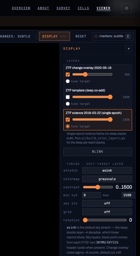
The toolbar
The display panel — Layers section
One row per image layer (see above), listed top-to-bottom in the order they're actually drawn — the change overlay is always the top row because it's drawn last. Each row has:
The display panel — Tuning section
These apply only to whichever layer is currently the tune target above:
The four panels around the edges
These are collapsed/out of the way by default so the sky stays the focus — each one is one click (or one hover, for the status line) away.
the full catalogue for this field
Click the ≡ button (or press L) to slide open a drawer listing every detection: search by id or verdict, filter by SNR / braai-pass / sign, include or exclude bogus, and sort. Clicking a row flies the view there and opens its detail drawer — the fastest way to browse rather than hunt for markers by eye.
which real survey shows as backdrop
Choose among a few real all-sky surveys (a colour photographic mosaic, the classic digitized plates, or a near-infrared survey) for whatever shows through when sky ctx is on or you zoom out past our field. The small i button explains what this layer is.
named real objects nearby
A collapsed panel that, once expanded, lists real catalogued astronomical objects (from SIMBAD) near the current view. Click one to fly there — useful for orienting yourself against something already known, independent of our own detections.
our catalogue, filtered to what's on screen
Like the sidebar list, but scoped to whatever is currently inside your field of view, sorted by signal-to-noise. Zoom in and more (fainter) detections are revealed, mirroring how you'd actually explore an image. Click a row for its detail drawer.
One more element, easy to miss: a small status line down the left-hand edge, above the sky-context panel, reports what just happened — load progress, a tuning change, or an error — and fades out on its own after a few seconds of inactivity.
The detection drawer
Clicking a marker on the map, or a row in the sidebar / nearby-detections list, slides a drawer in from the right with everything known about that one detection:
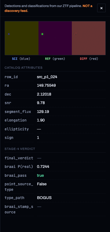
src_p1_024) — thumbnail, catalog attributes, and the Stage-4 classification verdict, exactly as the pipeline produced them.- · A repeat of the honesty banner, so the framing travels with the data.
- · The detection's own cutout — a small square of real sky at that exact position, with a caption naming each panel it holds (science, reference, difference, or whichever of those exist for that exposure).
- · Catalog attributes: sky position, signal-to-noise, sign, shape (elongation), and more.
- · The classification verdict: the real/bogus gate's pass/fail and confidence, an object-type call if one was made, and the pipeline's final verdict — with any uncalibrated probability struck through and any branch that never ran reading not run rather than a silent "bogus."
Close it with the × button, Esc, or by clicking anywhere outside the drawer.
Cutouts: the pixels behind every detection
Every detection in the application now carries its own cutout — a small square of real sky, cut straight from the images the measurement was made on, centred on that detection's own position. It is the fastest way to check a number against reality: a row can claim SNR 500, but the cutout shows you whether that is a star, a streak, or a subtraction artifact.
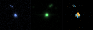
src_p1_010, a catalogued variable
star) — science, reference,
difference, left to right. The star is present in both
images; the difference panel shows what changed between them.The panels, and why there may not be three
The caption under a cutout always names the panels it actually has, and it will not always say three. Most of the harvest was run in a motion-only mode that never downloads a science frame, so a great many detections have a reference + difference pair, and some have the difference alone. That is a statement about which images exist for that exposure, not about the quality of the detection — read the caption rather than assuming a fixed triplet.

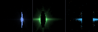
Reading one
- Left to right is a story. Before, after, and what the subtraction made of the pair. Look at the difference panel last, once you know what was there to begin with.
- Compare the two sky panels first. If the source is obviously brighter or fainter in one, the change is real. If they look identical but the difference panel is loud, the subtraction is what is loud — suspect a dipole.
- Judge the difference panel's shape, using the four shapes in section 04: compact blob, line, dipole, or saturated core.
- Trust the scale. Every panel of every cutout in an exposure is stretched by the same measured noise level of the whole frame — not by its own brightest pixel — so a faint residual looks faint and two cutouts can be compared honestly against each other.
- Then read the verdict beside it. The picture and the classification are two independent opinions; a cutout that looks nothing like a star is a good reason to distrust a confident-sounding label.
Each panel is 63 × 63 pixels — the same stamp size ZTF puts in its own public alerts — and is cut by sky coordinates, so all the panels land on the same star even though they come from different nights and different pixel grids.
Where to click for one
Reading a detection
The handful of terms that show up on every marker, row and drawer.
Mouse & keyboard
Troubleshooting
You opened the file directly
(file://). The viewer fetches its imagery and catalogue over HTTP, which browsers
block for local files. Run ./serve.sh from the project root and open the printed
address instead.
That's usually correct — empty sky is deliberately rendered true black. If the field itself looks empty, check the display panel's Layers list: a layer may be unchecked or its opacity down at 0%. Try reset in the toolbar to restore every default.
Markers only exist inside this page's one baked field/exposure (named in the strip at the top). If you've panned far away, fly back with reset, or open the ≡ sidebar and click any row to jump straight to it.
Blink needs both a sky layer and the deep template layer present. If either is missing on this build, a status message names which one — check the status line down the left-hand edge right after clicking.
It's synthetic two-band colour (ZTF g+r only), not a real three-filter photo and not Rubin data — see What you're looking at. If only one band was built, you'll see grayscale instead, and the Layers panel will say so explicitly.
Normal on first load: the viewer boots on the wide real sky, then flies in to the ~0.86° ZTF field once imagery has arrived — give it a few seconds before judging the picture.
Ready to open it
You now know every panel on the page. Open the viewer, or zoom out first to the wider harvest this one field sits inside.
open it now
every patch we've harvested
every exposure, on the sky
what this pipeline actually is
the "why" behind what you're seeing